Next, the process for generating the Nordic typology and the operational steps taken are described and discussed. Figure 5 illustrates the different phases of work, including the pre-analysis phase as well as the steps for constructing the urban and the rural typology classes. A more detailed discussion of the different work stages and key considerations at each phase are provided in the following. 

Data and methods 

The Nordic typology was constructed using an approach that relies on a combination of both traditional geographic information system (GIS) methods as well as machine learning. The overlap between these two approaches provided the opportunity, upon review of both methods and results, to proceed using a strategy that produced the more accurate results. Thus, it was concluded that traditional GIS methods would provide a firm background with less risk. Machine learning, on the other hand, provides benefits, but with some inherent uncertainty. A combination of both approaches was ultimately adopted for exploring how a Nordic urban–rural typology could be produced using (predominately) openly available data. 

The Finnish typology was used as a starting point and as a reference classification for constructing the Nordic typology. An important way of assessing the initial results and to adjust the model was to compare how well the typology classes, generated using the combined GIS and machine learning-based approach (with open data), corresponded to the Finnish urban–rural classification. 

Table 2 lists the key data used for generating the Nordic typology. The work was initiated by obtaining national spatial grids (1 x 1 km) including data on population from each of the five Nordic countries, obtained from the National Statistics Institutes of each country. At this stage, experiments to disaggregate population statistics from the municipality level to grid level were also made. While these experiments were not included in the final model, they nevertheless demonstrated the possibility of estimating grid-level population based on annual municipal population statistics, which could possibly be applied in the future. 

Data on buildings from the different Nordic countries was regarded as important for generating the typology. Here buildings were classified into three classes based on the number of floors (apartment buildings with 1–2 floors, apartment buildings with 3 or more floors, other buildings). These datasets were not uniform and, for Iceland, the classification of buildings was based on estimates from OpenStreetMap, which resulted in less accuracy. On the other hand, an advantage of using OpenStreetMap data was that it was possible to reproduce building classification for the other countries. Additionally, European CORINE land-cover data were used to generate the typology classes based on which land-use class was most prevalent in each grid (see also the next section). 

Table 2. Data used in generating the Nordic Typology. 

Classification experiments 

In the initial stages of work, there was an assumption that it would be easier to predict the urban typology classes from the available data, compared to the rural classes. As the main challenge was expected to be in detecting different types of rural areas, it was decided to follow an experimental approach, using the Random Forest technique. Essentially, Random Forest is a supervised machine-learning classification algorithm that can be used for classification purposes. This approach was tested on one of the rural classes in Finland, namely, rural heartland areas, where this specific class was taught to the classifier, to see how well the areas identified using this technique corresponded to the areas defined as rural heartland in the Finnish typology. The results proved to be so robust that it was decided to broaden the scope of this approach and to attempt to identify all classes using this method. 

The outcomes of the Random Forest classification, applied to all classes in Finland, were compared to the original Finnish classification. The overall result was satisfactory and corresponded relatively well to the original classification. While some minor misclassifications and errors were present, it was considered possible to mitigate these errors at later stages of the work. 

At this stage, the following data (at 1 x 1 km grid level) were used: total population, number of ‘low’ residential buildings with one or two storeys, number of ‘high’ residential buildings with three or more storeys, and the number of unknown buildings. The aforementioned building data were open-source data from the Topographic Database of the National Land Survey of Finland (NLS, 2023). One observation was that some systematic classification errors had occurred inside larger lakes at this stage, and that these misclassified areas were typically uninhabited and did not contain any buildings. To address this issue, it was evident that there was a requirement to also including a variable for land use, to obtain a more reliable classification. An advantage of the incremental design approach used was that it allowed for experimenting with the model and adapting it easily by further including land-use data as well.  

It was also decided to include European CORINE land-cover data, which includes 44 hierarchically structured land-use classes (EEA, 2023a). The most exact land-cover classification was used, and the data were then generalised into a 1 x 1 km grid. As all land-cover classes were not necessarily present in all countries, this required careful handling, and meant that if a certain land-use variable was present in a specific country but not included in the model, the feature was then excluded. 

Country-specific considerations 

As described, in the early phases, the model was fitted using Finnish data to identify the robustness of the model as well as any needs for improvement. It was, however, still uncertain at this stage how well the model would perform for the other Nordic countries. To assess this, it was necessary to gather source data and compute aggregates for the other countries. In attempting to obtain data from all the Nordic countries, there were several challenges and considerations regarding data that had to be acknowledged and addressed. These included uncertainty about what data were available from the different countries for specific reference years. Another issue was that data classifications may differ between countries, which was the case with the building data, for example. Additionally, the documentation of data is not always available (or up-to-date), adding uncertainty regarding the quality of this input information.  

 

Approaching the final classification 

As already outlined, the Random Forest approach was used for classifying all seven typology classes that exist in the Finnish urban–rural classification. While this approach provided satisfactory results, there remained a requirement to have greater control of the final classification, and hence a two-class rural classifier was developed. This meant creating a uniform countrywide canvas for the two classes: rural heartland and sparsely populated rural, for all Nordic countries. Following this is it was necessary to compute all the other classes using traditional GIS methods. Slight adjustments were made to the model’s learning material by including urban areas inside rural areas, to then be able to create a continuous canvas (without gaps) on top of which the actual urban classes could be overlaid. 

The identification of urban centres was done using a separate classifier, which was fitted for Finland using the original Finnish urban–rural classification as reference data. This involved aggregating the original urban centre source data to 1 x 1 km grid cells and using the result for fitting the classifier. Here, population and building data aggregated to the grid cells were used in the model as features, and the Random Forest approach was used once again. This resulted in contiguous urban centres with populations of 15,000 inhabitants or more. 

In the original Finnish typology, labour mobility is modelled according to the Herfindahl index (see e.g. Eurostat, 2021) and using data on commuting and economic and labour market data structures. However, it was not possible to use a similar approach for the Nordic typology owing to a lack of openly available data from all the Nordic countries. Instead, it was decided to test two alternative approaches, namely, Huff gravity modelling for each centre, along with a fallback approach where travel-time isochrones were computed to show accessibility to urban centres. The Huff model allowed comparison of urban centres and their relative accessibility with other centres. Experiments were carried out for Denmark using this approach. However, as these computations were highly time consuming (and their added value was uncertain) it was instead decided to proxy the missing travel-time data with isochrone computations. 

In the following, a closer look is taken at the operational steps for generating the seven territorial classes of the Nordic urban–rural typology. The focus is first on the main steps for creating the urban typology classes, followed by the rural classes. These steps follow the process presented in Figure 5. 

 

Delineating urban settlements 

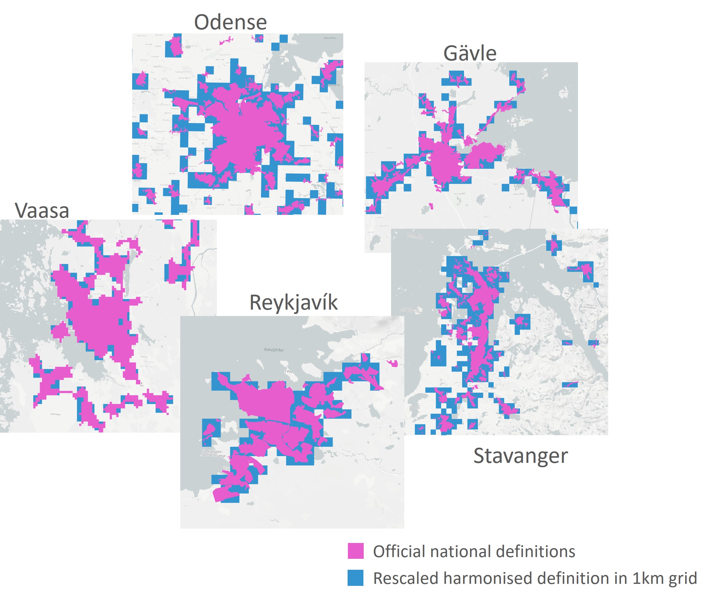
To generate the urban classes in the typology, a key starting point was to first delineate urban settlement areas in all five Nordic countries. Each Nordic country has its own official definition of urban settlements (tätort (SE), byområde (DK) taajama/tätort (FI), Þéttbýlisstaður (IS), tettsted (NO)) and provide data corresponding to these definitions. The definitions are similar in all the Nordic countries where urban settlements are defined as places where 200 persons live within 200 m (in Norway 50 m) of each other. For the development of the urban classes in the Nordic typology, a first step involved harmonising urban settlements across all five Nordic countries. This was achieved by estimating and scaling the Finnish urban settlement definition, originally generated using a 250 × 250 m grid, into a 1 x 1 km grid and then adjusting the result based on observations from the other countries (see Figure 6). 

More specifically, the results were adjusted according to the following steps. First, based on the population and building densities of a 250 × 250 m grid cell in Finland, the urban classifier was taught to classify these grid cells as either urban or non-urban. This was a necessity since building and population register data were not available for all countries. The 250 m classifier was first validated against the boundaries of the official delimitation of urban settlement areas (taajama/tätort) in Finland. At this stage the classifier estimated, with an accuracy of 250 m, whether grid cells were part of an urban settlement based on the population and number of buildings contained therein. While the 250 × 250 m grid-level urban classifier worked well, for the purpose of the typology, it was necessary to scale it to the 1 × 1 km grid level; this step first involved testing the 1 × 1 km urban classifier in Finland. The final model was not well suited to a direct scale up the population and building densities (250 × 250 m to 1 × 1 km grid level). This was because of the much larger areas covered by the 1 × 1 km grid, which meant that the scaling became too inaccurate because the larger grid size does not sufficiently follow the actual boundaries of built-up areas. The sensitivity of the urban classifier used to form 1 × 1 km grids was therefore adjusted using observations and calculations. The final classifier result was refined using an iterative process using a selection of criteria (i.e., using information based on the total area differences between alternative delineations of urban settlements as compared with the official delineations of the different countries within the group). 

For the final model, the option that generated the smallest difference using the official delimitations of all the countries was selected. The final classifier, therefore, took account of the data for a single 250 × 250 m grid cell and the proportion of the area of the 250 × 250 m grid cells that were classified as urban settlements within the 1 × 1 km grid cells (using a 5 x 5 focal analysis circle). The area of the 250 m grid cells covered at least 50% of the area within the larger grid cells. 

Identifying urban regions 

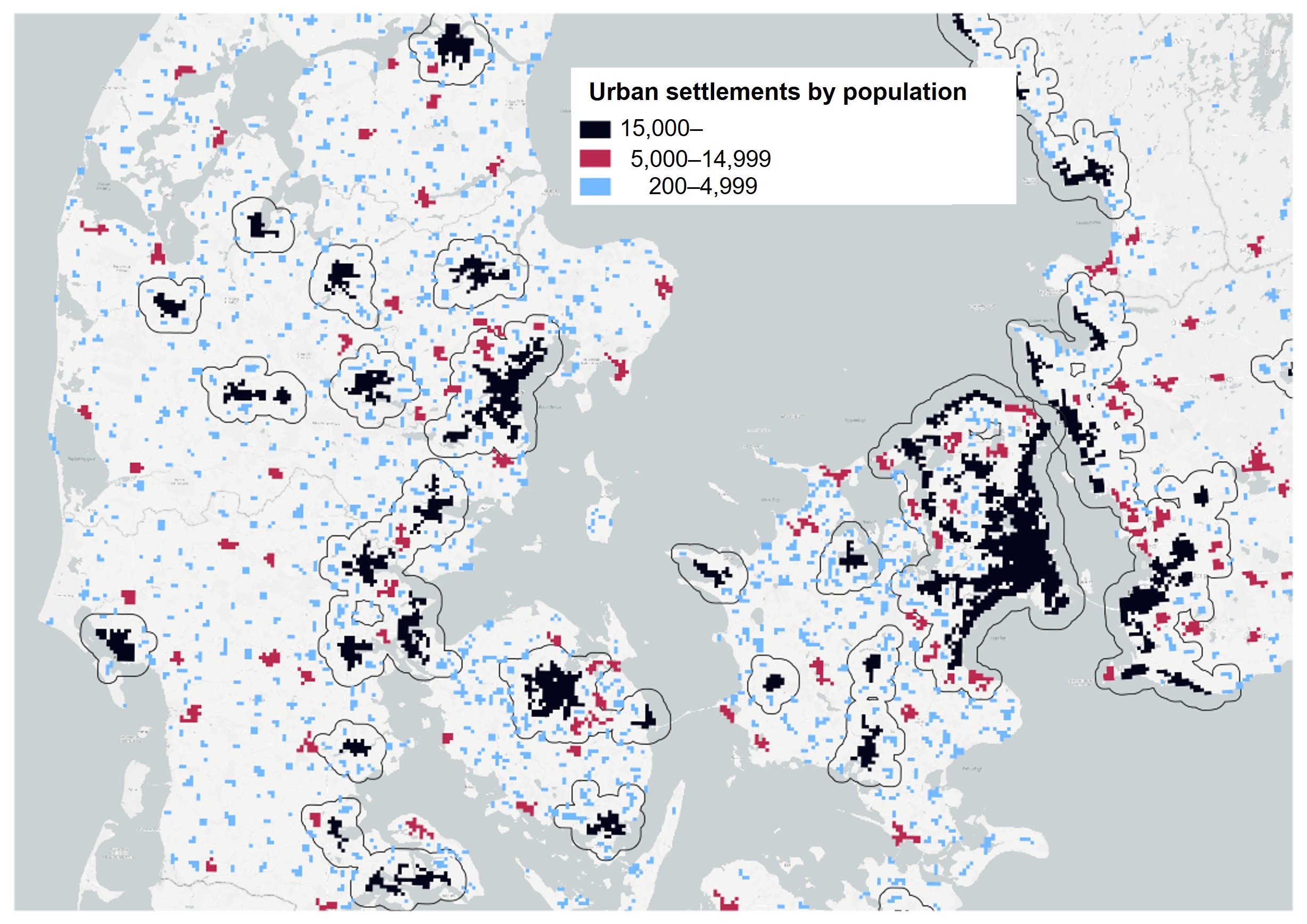
Following the delineation of urban settlements in all the Nordic countries, the next step involved identifying territories that could be defined as urban regions. Here, urban regions were defined based on those urban settlements having a population of more than 15,000; marked by boundaries showing the extent of these regions (see Figure 7)¹. This meant that the urban regions identified include both the urban settlements as well as their surrounding areas. Smaller settlements with fewer inhabitants, located near the central urban settlement and situated within the previously delimited urban regions, were then defined as neighbouring settlements (provided that the settlement areas touch a 3 km buffer region of those urban settlement areas with over 15,000 inhabitants).  

A three-tier classification of urban settlements can be seen in Figure 7. In this map, urban settlements with more than 15,000 inhabitants form the core settlement areas (keskustaajama/centraltätort) within urban regions (marked black). Urban settlements with a population in the range 5,000–15,000 (marked red) are considered local centres in rural areas if they are located outside the boundaries of urban regions. Urban settlement areas with fewer inhabitants (marked blue and red) can extend the boundaries of urban regions if these smaller settlements are located sufficiently close to the core settlement areas (within a 3 km radius). 

^{1 This work was based on the delineation of urban regions in the Finnish Monitoring System of Spatial Structure and Urban Form (YKR). For a more detailed description of the methodology for see SYKE (2023).} 

Figure 7. Classifying urban settlements by size and generation of urban regions.  

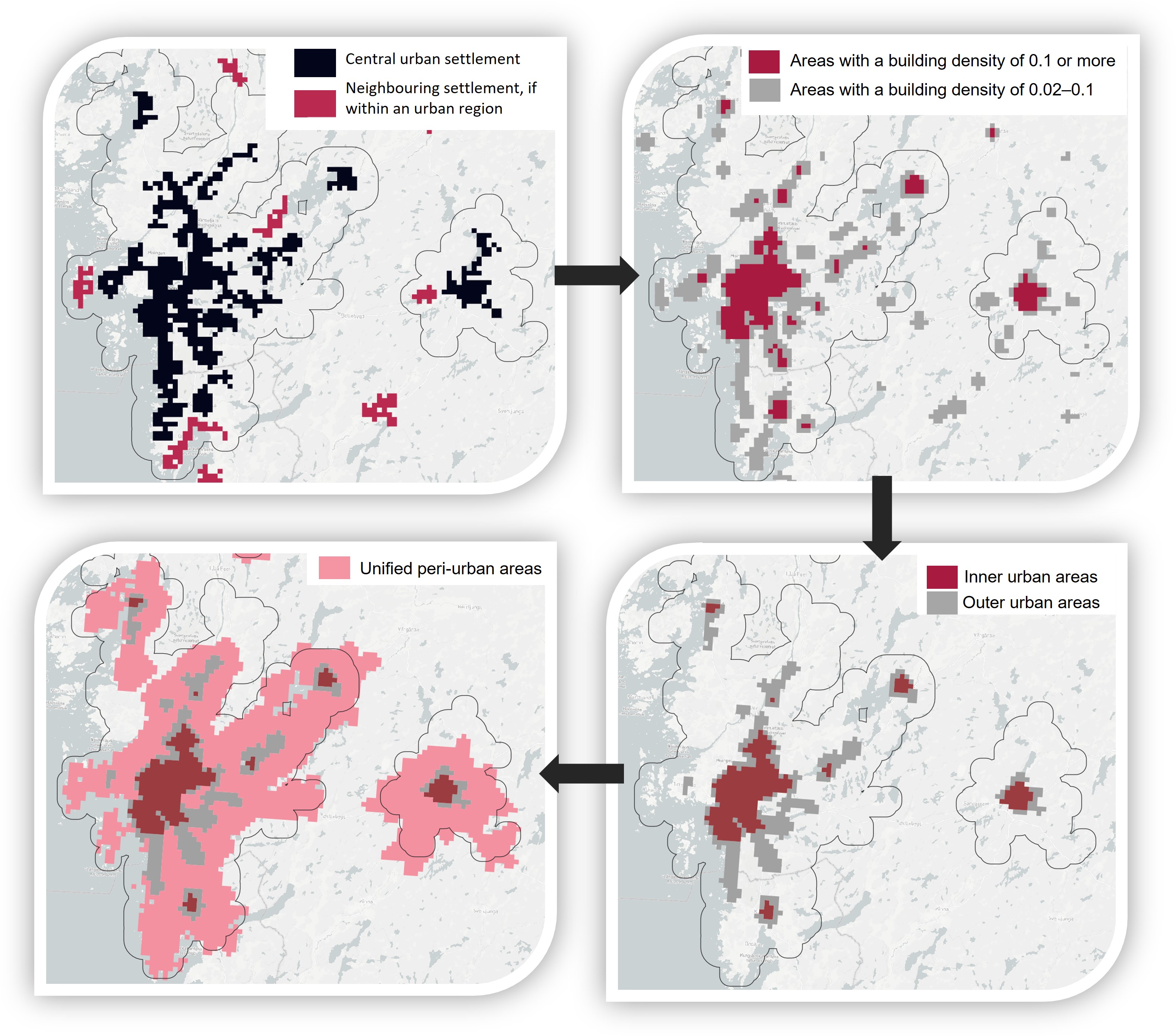
The steps for delineating urban areas and defining the different urban typology classes are illustrated in Figure 8. Having identified central urban settlements and neighbouring settlements within urban regions, the next step involved defining the built environment of these areas according to building density (or floor-area ratio). This was done using proxy-estimates from population and building data. Depending on floor-area ratio (calculated as the floor area of buildings in relation to the size of the urban area), areas were classified as either ‘inner urban areas’ (with a floor area ratio of 0.1 or greater) or ‘outer urban areas’ (having a floor area ratio between 0.02 and 0.1). For this step, a circular 3 × 3 focal analysis was used for generating the final polygons for inner and outer urban areas. This was followed by defining and delineating peri-urban areas that surround the inner and outer urban areas, based on accessibility calculations to the centre of the urban region. Here, generalised 6-minute travel-time zones were calculated around the outer urban areas and 4.5-minute travel-time zones were calculated around smaller urban settlements, resulting in a layer of unified peri-urban areas. 

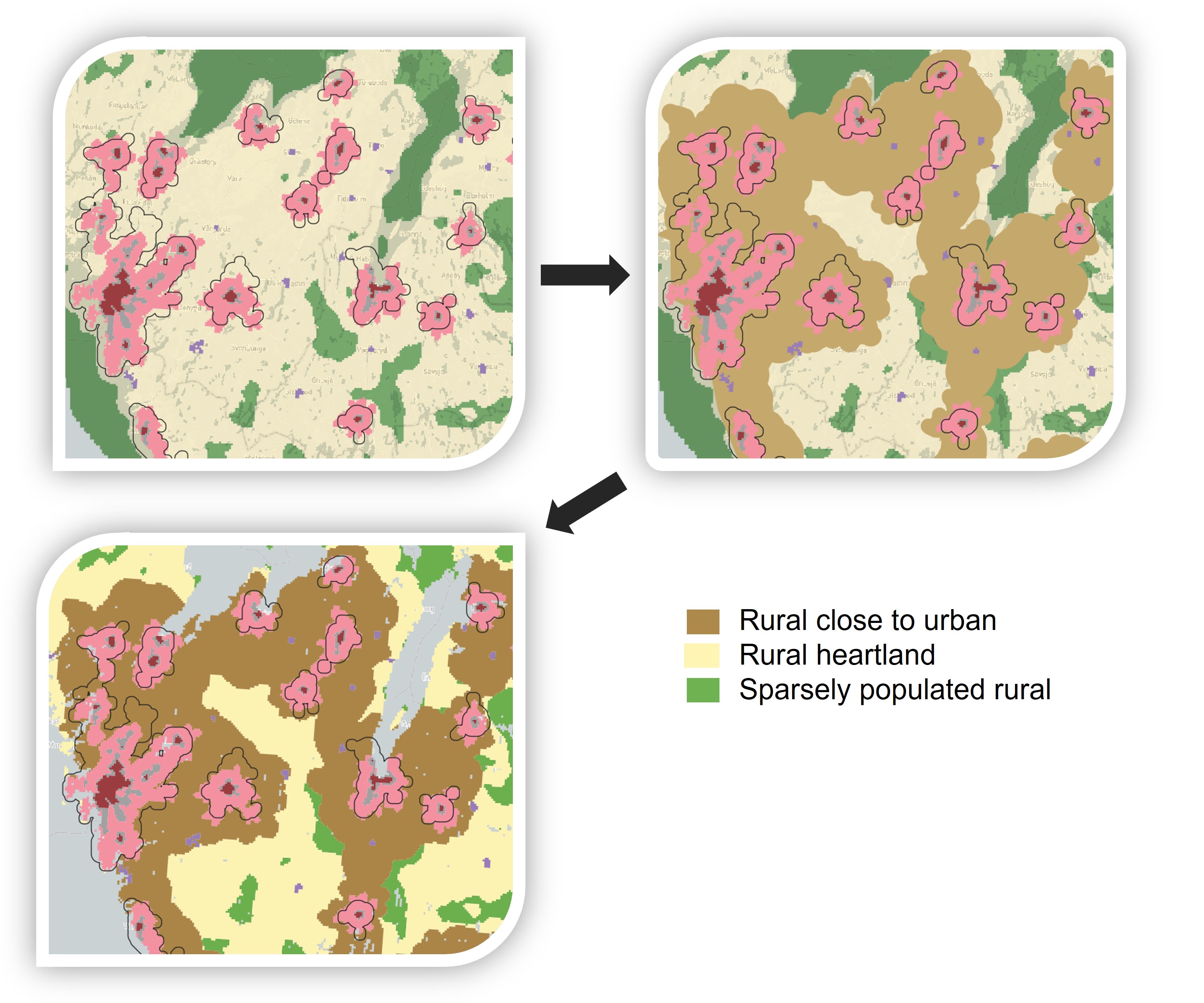
In generating the rural typology classes, the first step involved identifying areas defined as local centres in rural areas. These areas were identified based on the previously generated urban settlements and by focusing on those settlements that are located outside the previously defined urban regions. Those urban settlements that did not form part of an urban region and had a population between 5,000 and 15,000 were classified as part of this class (red areas in Figure 9). 

 

Figure 9. Local centres in rural areas (urban settlements located outside urban regions with a population of 5,000– 15,000).  

The remaining rural classes in the typology were created based on population, building density, and land-use intensity estimations derived from CORINE land-cover data. The steps taken are shown in Figure 10 and were achieved by teaching an AI model, based on the Finnish urban–rural classification, to classify rural areas into either rural heartland or sparsely populated rural areas. Areas with a rural character that are functionally connected and close to urban areas were conceptualised as ‘rural close to urban’; estimated based on generalised travel-time and distance estimates from the urban core. The area depends on the size and distribution of the urban area and on the connectiveness between two or more urban areas. The areas that form this typology class are characterised by an average driving time of 20–30 minutes from the edge of outer urban areas.  

This stage of the work involved testing, on a step-by-step basis, the most suitable way of using travel-time isochrones calculated from urban settlement areas of different sizes. The result used a multi-step travel-time calculation combined with calculating buffer zones. The final model used travel-time calculations with a 10–24-minute interval. The use of travel-time isochrones was weighted by the population size of the settlement area such that the larger settlement areas had a longer range of influence than smaller settlements. 

 

Figure 10. Operational steps for delineating the rural typology classes.   

The process diagram in Figure 5 shows the steps that were followed to create the Nordic urban–rural typology. The key steps are summarised as follows: 

 

The typology developed through the previously presented steps classifies Nordic territories into seven different classes. Figure 11 shows the framework for how the Nordic urban–rural typology and its different territorial classes can be understood in relation to each other. 

 

Figure 11. Framework for the Nordic urban–rural typology and its different typology classes, based on the Finnish urban–rural classification (Helminen et al. 2014).  

A brief explanation of the key characteristics of the different typology classes is defined below. 

Figure 12 shows a comparison of how territories in the five Nordic countries are classified in the new grid-based urban–rural typology compared to the Eurostat DEGURBA typology. The most noticeable differences can be seen in municipalities that are vast in size, for instance in the northern parts of Finland, Norway, and Sweden. While these municipalities and their entire territory are classified as either predominantly rural, intermediate, or urban in the DEGURBA classification, according to the Nordic typology, there are clear territorial differences within these municipalities, which include various areas that belong to several of the different territorial classes of the typology. 

The Nordic urban–rural typology has also been published on an interactive digital web-mapping platform where the typology can be better visualized and where it is possible to zoom in on different areas across the Nordic countries (see Figure 12). The interactive version of the typology can be accessed online from where it can also be downloaded for further use.   

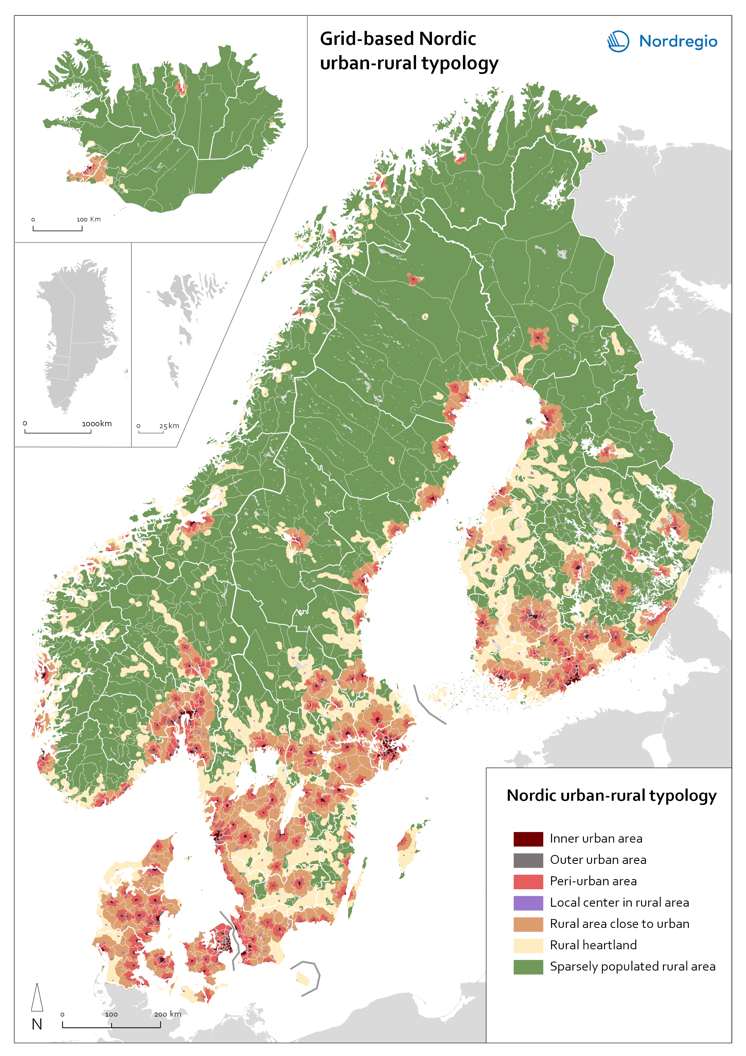
 Figure 13. Comparison of how territories are classified in the Nordic urban–rural typology and in the DEGURBA classification.